Quick start tutorial

This tutorial will quickly walk you through the basic functionality of GLINT. For this tutorial we use subset of a public dataset from GEO (accession ID GSE77716; the dataset is described in details in Rahmani et al. [1]). In order to run this tutorial you will need to download GLINT and get the tutorial files (see here).

The tutorial files include:

• datafile.txt - 50,000 sites by 96 samples matrix of methylation levels
• covariates.txt - covariates matrix, each column corresponds to one (numeric) covariate
• phenotypes.txt - phenotypes matrix, each column corresponds to one phenotype

Bellow is a set of simple commands, together composing a full pipeline of EWAS analysis (after raw data normalization). The commands bellow assume the user downloaded GLINT (see Download and installation) and added the tutorial files into the software's root directory. For more details about any specific argument see the documentation.

Note

Avoid execution errors by using the latest release of GLINT and the tutorial files, and make sure to follow the installation instructions in the README file.

1. Create GLINT files

First, we start by saving a binary version of our data: the methylation data file, covariates and phenotypes of interest. This step will allow a substantial speed-up in all following commands. Navigate to the GLINT directory and run the following:

python glint.py --datafile datafile.txt --covarfile covariates.txt --phenofile phenotypes.txt --gsave

The output of this command is the file datafile.glint, a binary version of the methylation data, and two additional files, datafile.samples.txt and datafile.sites.txt, providing textual information about the samples and sites in the data.

2. Detect outliers

We begin the analysis by looking for outliers in the data. We first run:

python glint.py --datafile datafile.glint --plot --plotpcs --numpcs 2 --out pcs_plot

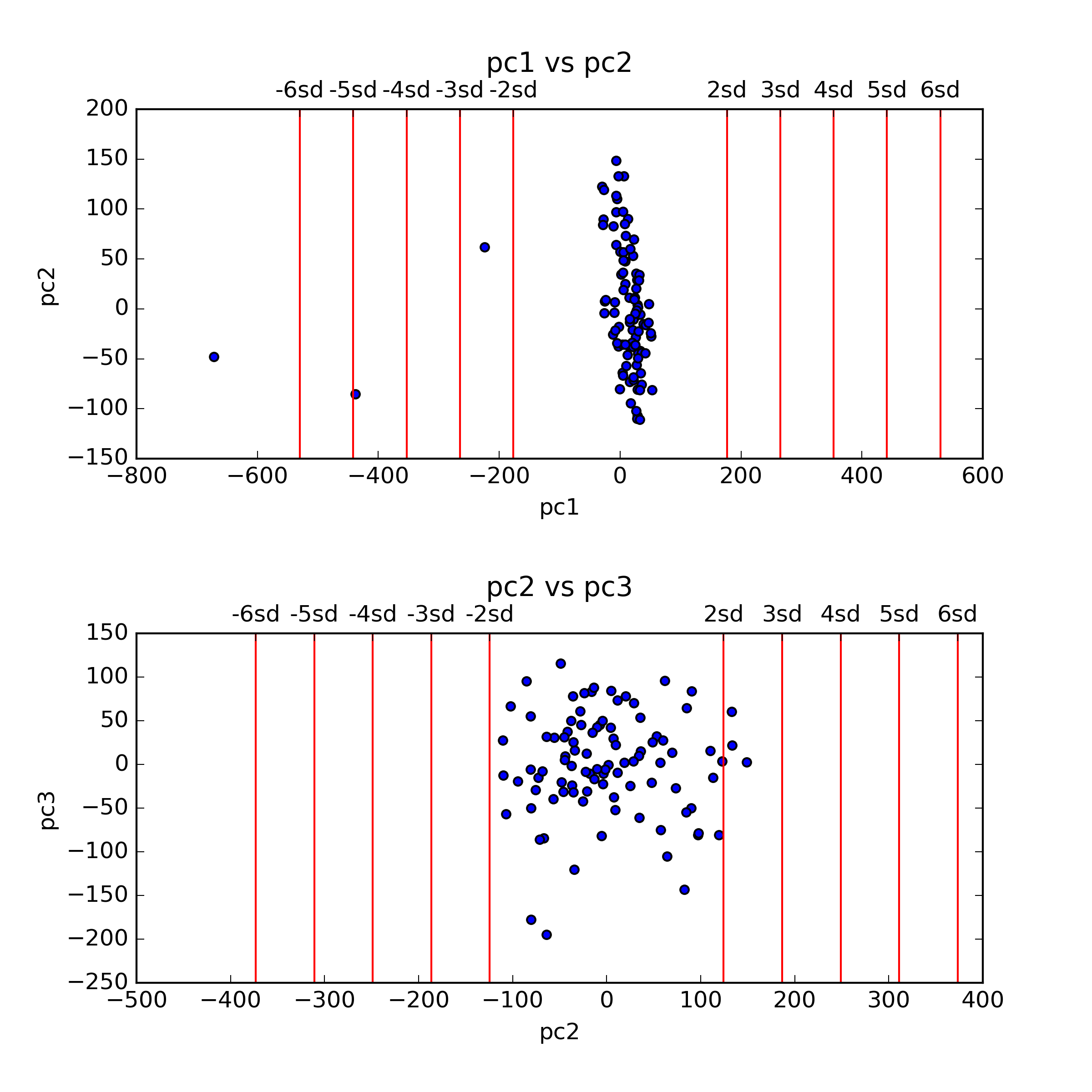
This command generates a figure titled pcs_plot.png, showing scatter plots of the first two principal components (PCs) of the data. Note that this command also generates an additional figure, pcs_plot.eps, a publication quality version of the same figure.

Note

For using `--plot`_ when working on a remote server (e.g., via SSH), make sure X11-forwarding is enabled.

3. Remove outliers

For this tutorial we consider samples with values more extreme than 4 sandard deviations (SDs) in their first two PCs as outliers. Following that definition, we currently have 2 outliers in the data, as reflected in the top panel of the pcs_plot.png figure. We remove these outlier samples by indicating 4 SDs as the maximum level allowed for PC number 1:

python glint.py --datafile datafile.glint --maxpcstd 1 4 --gsave --out data_cleaned

As before, we use the --gsave argument for generating GLINT files, only this time with outliers excluded. This results in the following files: data_cleaned.glint, data_cleaned.samples.txt and data_cleaned.sites.txt files.

4. Capture cell type composition

Since our data were collected from a heterogeneous source (blood tissue), we run ReFACTor in order to account for the cell type composition in the downstream analysis and generate new GLINT files with the results. The resulted ReFACTor components will be used later as covariates in our EWAS analysis, as tissue heterogeneity is a potential confounder in EWAS [2]. In order to boost ReFACTor's performance in capturing the cell composition, we run ReFACTor while adding potential methylation altering factors as covariates. We do that by using the --covar argument which allows us to add covariates by their names (as they appear in the covariates file):

python glint.py --datafile data_cleaned.glint --refactor --k 6 --covar age gender chip1 chip2 chip3 chip4 chip5 chip6 chip7 chip8 --gsave --out data_cleaned_v2

This command creates data_cleaned_v2.refactor.components.txt and data_cleaned_v2.efactor.rankedlist.txt files (see Tissue heterogeneity for more details), and updated GLINT files: data_cleaned_v2.glint, data_cleaned_v2.samples.txt and data_cleaned_v2.sites.txt. Note that data_cleaned_v2.samples.txt includes new covariates: rc1, rc2, ..., rck - these are the ReFACTor components.

5. Infer population structure

Since our data were collected from admixed population and we do not have ancestry information available, we estimate the population structure in the data directly from the methylation levels using the EPISTRUCTURE algorithm [3] and generate new GLINT files with the results. In order to boost the performance of EPISTRUCTURE in capturing the ancestry information, we run EPISTRUCTURE while adding strong genome-wide effectors as covariates - in our case we add the estimates of the cell composition. The resulted EPISTRUCTURE PCs will be used later as covariates in our EWAS:

python glint.py --datafile data_cleaned_v2.glint --epi --covar rc1 rc2 rc3 rc4 rc5 rc6 --gsave --out data_final

This command results in a file titled data_final.epistructure.pcs.txt (see Inferring population structure for more details). In addition, we now have data_final.glint, data_final.samples.txt and data_final.sites.txt files. Note that data_final.samples.txt includes a new covariate named epi1, which is the first EPISTRUCTURE component (by default --epi outputs one component).

6. Run EWAS

We are now ready to run association test for each site. In this tutorial we will run EWAS on a simulated phenotype. The phenotype is selected using the --pheno argument, according to the phenotype's name in the phenotypes file. Since our phenotype is continuous we will use a linear regression model, and in addition to standard age and gender covariates, we will include the ReFACTor components and the first EPISTRUCTURE component in the analysis in order to account for tissue heterogeneity and population structure. In addition, using the --stdth argument we can neglect nearly constant sites having very low variability, and using the arguments --rmxy, --rmns and --rmpoly, we can also neglect X and Y chromosomes sites, cross-reactive sites and polymorphic sites [4].

python glint.py --datafile data_final.glint --ewas --linreg --pheno y1 --covar age gender rc1 rc2 rc3 rc4 rc5 rc6 epi1 --stdth 0.01 --rmxy --rmns --rmpoly

This command outputs a file titled results.glint.linreg.txt with the results of the association test. Note that the results are sorted by their association p-value.

7. Plot results

Lastly, we would like to plot the results in the results.glint.linreg.txt file. GLINT allows to visualize the results by plotting a qq-plot (--qqplot) and a Manahattan plot (--manhattan) as follows.:

python glint.py --plot --qqplot --manhattan --results results.glint.linreg.txt

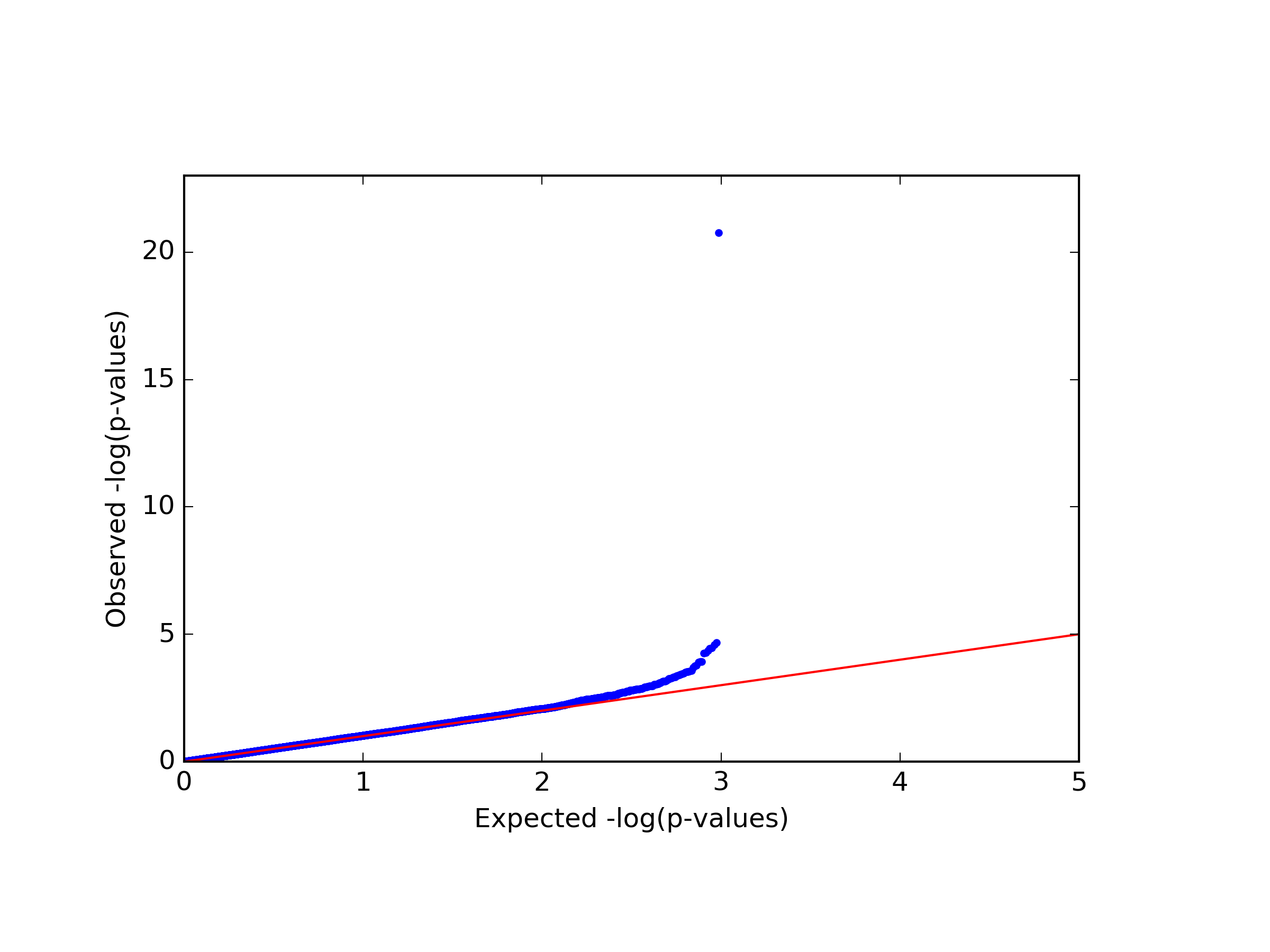
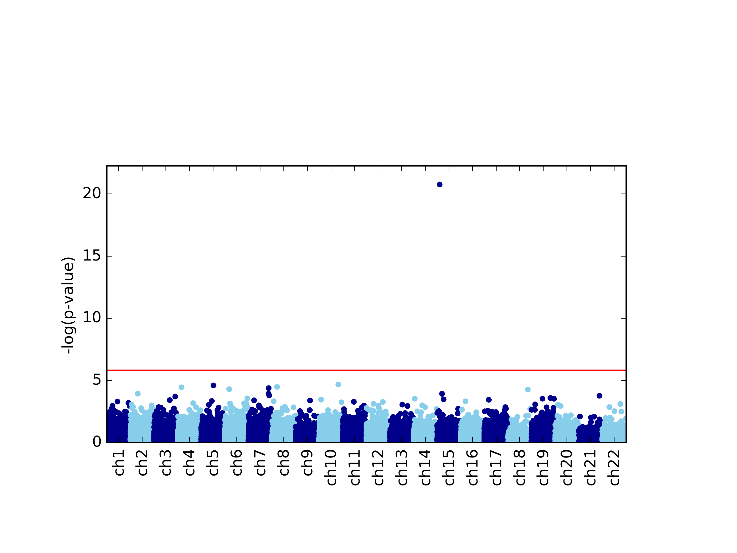
This command generates four figures. The first two, results.glint.qqplot.png and results.glint.manhattan.png, show a qq-plot and a Manhattan plot of the results. The last two are publication quality versions of the same figures (.eps files).

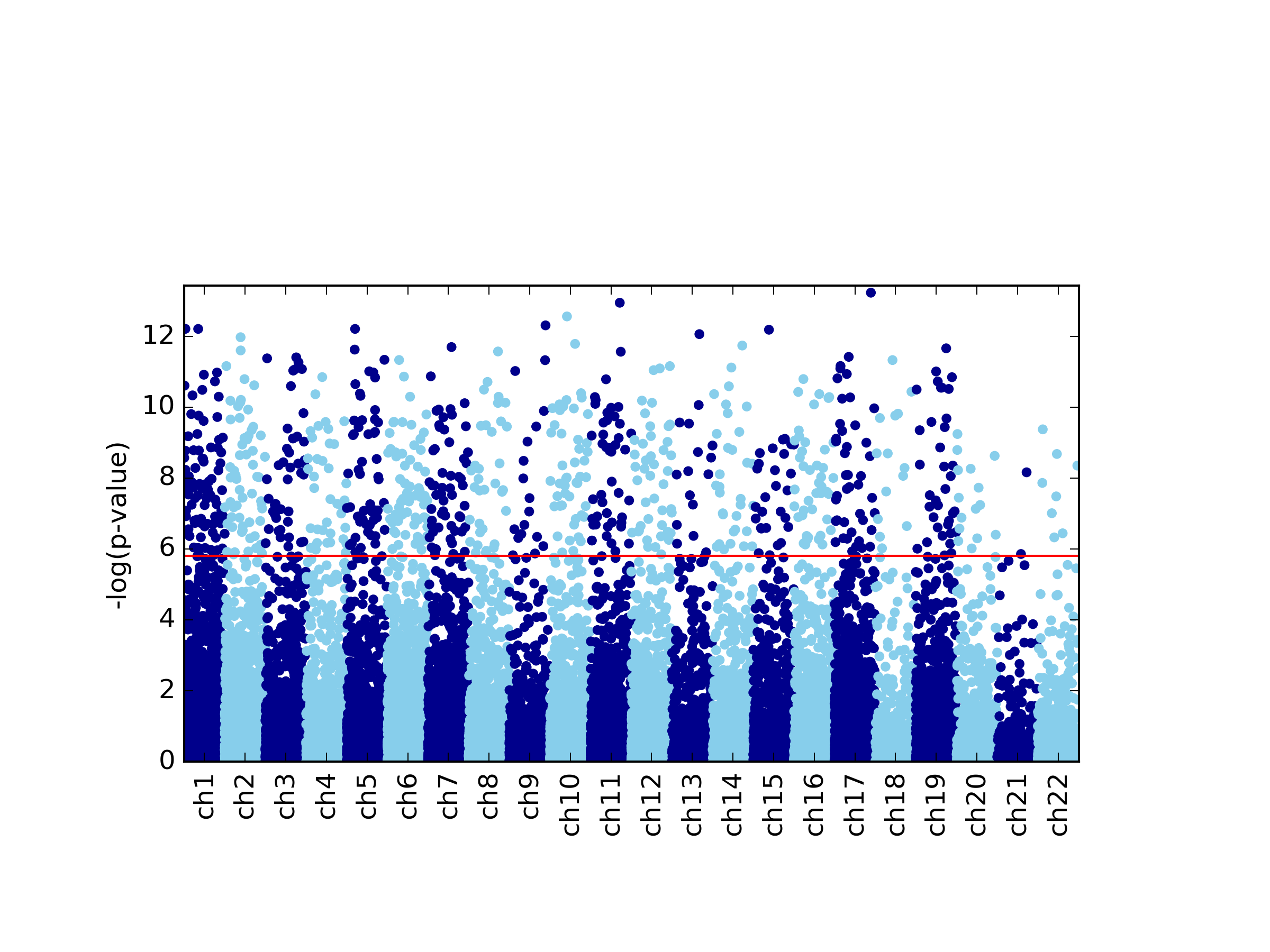
8. Unadjusted EWAS

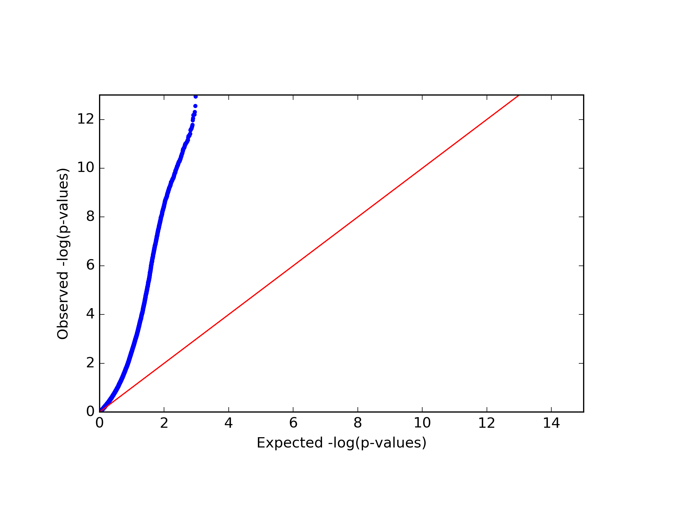
Finally, in our example we found a single significant association in chromosome 15 (cg20510272), as reflected in the qq-plot and in the Manhattan plot. The phenotype we used here was simulated to be correlated with the cell type composition in the data and only one site (cg20510272) was artificially changed to be causal with respect to the phenotype. Since the phenotype is correlated with the cell type composition, performing uncorrected analysis is expected to result in many spurious assocaitions. We can easily see that by running an unadjusted EWAS by simply repeating our EWAS analysis, this time without including the ReFACTor components as covariates. Here, we use a single command for running the EWAS analysis and generating the plots at the same time:

python glint.py --datafile data_final.glint --ewas --linreg --pheno y1 --covar age gender epi1 --stdth 0.01 --rmxy --rmns --rmpoly --plot --qqplot --manhattan --out unadjusted

[1]	Rahmani, Elior, Noah Zaitlen, Yael Baran, Celeste Eng, Donglei Hu, Joshua Galanter, Sam Oh et al. "Sparse PCA corrects for cell type heterogeneity in epigenome-wide association studies." Nature methods 13, no. 5 (2016): 443-445.

[2]	Jaffe, Andrew E., and Rafael A. Irizarry. "Accounting for cellular heterogeneity is critical in epigenome-wide association studies." Genome biology 15, no. 2 (2014): 1.

[3]	Rahmani, Elior, Liat Shenhav, Regev Schweiger, Paul Yousefi, Karen Huen, Brenda Eskenazi, Celeste Eng et al. "Genome-wide methylation data mirror ancestry information." bioRxiv (2016): 066340.

[4]

Chen, Yi-an, Mathieu Lemire, Sanaa Choufani, Darci T. Butcher, Daria Grafodatskaya, Brent W. Zanke, Steven Gallinger, Thomas J. Hudson, and Rosanna Weksberg. "Discovery of cross-reactive probes and polymorphic CpGs in the Illumina Infinium HumanMethylation450 microarray." Epigenetics 8, no. 2 (2013): 203-209.